The first post in this series showed the importance of the glass transition temperature (Tg) versus fractional conversion to correlate the development of Tg as a function of thermoset curing. One relatively easy and straightforward method to build the Tg-conversion plot is to use differential scanning calorimetry (DSC).
The first task is to determine the ultimate glass transition temperature, termed Tg∞. To determine Tg∞, prepare an uncured sample in a DSC pan and crimp using the equipment manufacturers sample preparation procedure. Heat the uncured sample at 10°C/min to above the end of the exotherm, but not too high to cause decomposition. After reaching the desired upper temperature, the DSC pan is quenched to sub-ambient (approximately -30°C) at a rapid cooling rate. Once equilibrated at sub-ambient temperature, the sample is subjected to a second temperature scan at 10°C/minute from sub-ambient to the appropriate upper temperature sufficient to measure the Tg. The second scan should exhibit an endothermic Tg and no residual heat of reaction should be observed. The Tg from the second scan is then assigned Tg∞.
An example of the DSC method is shown in Figure 1.
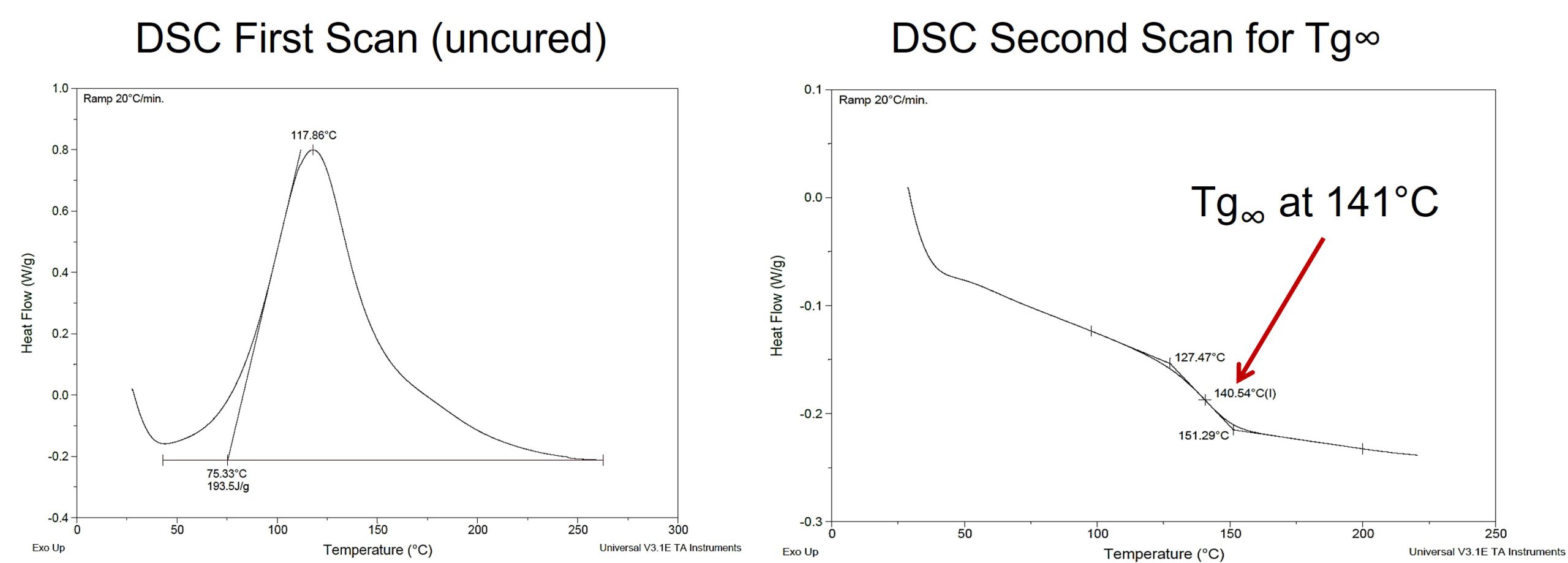
Figure 1. DSC traces showing the two-scan method to determine Tg∞ for an epoxy-amine.
The DSC trace on the left shows the first scan of the uncured epoxy-amine where the total heat of reaction, ΔHrxn was measured. Note the temperature was ramped to 250°C where the exotherm ended. After cooling to room temperature, the DSC curve on the right was obtained and the Tg∞ was measured to be 141°C.
Once Tg∞ is known, then several isothermal temperatures may be chosen. An example is shown in Figure 1, where the DSC traces are displayed as a function of cure time at 160°C for another epoxy-amine curing system [1].
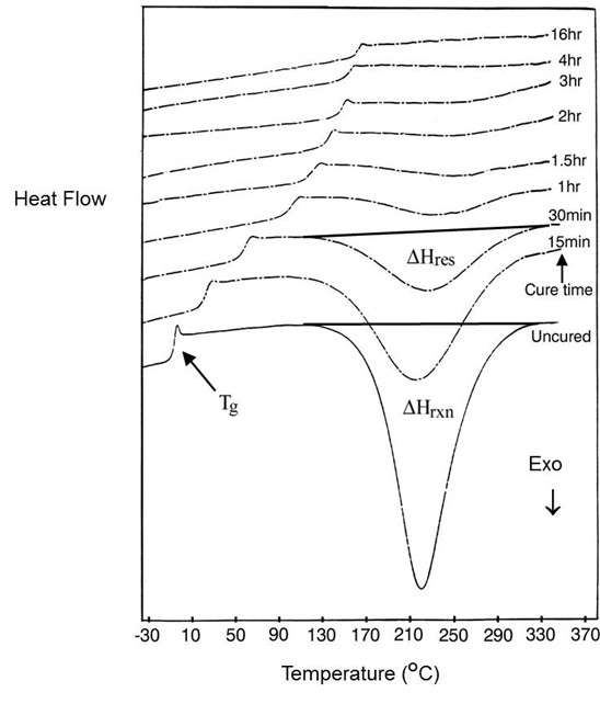
Figure 2. A series of DSC temperature scans at 10°C/min of an epoxy–amine cured isothermally at 160°C for different times. From [1]
From DSC measurements, the conversion or degree of cure at time t, αt, is defined as:
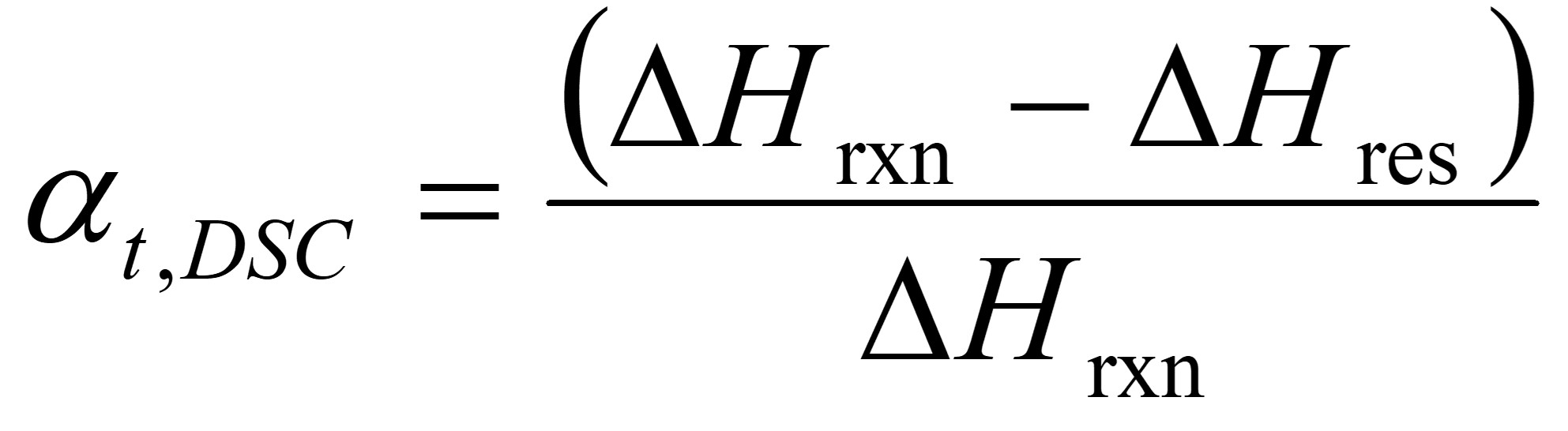
where ΔHres is the residual heat of reaction at time t.
Figure 2 contains DSC scans of epoxy-amine cured at 160°C for various times between zero and 16 hours. Each scan showed Tg and the residual cure exotherm ΔHres. For the time zero curve the exotherm is the total heat of reaction ΔHrxn. Conversion α at each time t, was calculated using the equation above.
To build the Tg-conversion plot, isothermal experiments at various temperatures below Tg∞ are required. A simple way to accomplish this is to mix a batch of the formulation you want to test and then place small amounts (approximately 10- 20 mg) of the mixed formulation into aluminum DSC pans. The number of DSC pans depends on how many cure times are required at each temperature. For example, in the data shown in Figure 2, nine (9) DSC sample pans were prepared (one for the uncured sample and 8 for the various isothermal curing times). After the sample is placed in the bottom aluminum pan, a lid is placed in the pan and crimped using the tool provided by the instrument maker. Once the DSC pans are crimped, they should be stored in a refrigerator until they are ready for the curing experiment.
The preferred way to conduct the curing experiments is to cure the sample pans inside the DSC under continuous nitrogen flow for the desired times. Isothermal curing should be carried out at specified temperatures above where the reaction initiates to slightly greater than Tg∞. After isothermal curing times in the DSC typically ranging from 10 minutes to up to 24 hours, each DSC pan is quenched from Tcure to sub-ambient (approximately -30°C) at a rapid cooling rate. Once equilibrated at sub-ambient temperature, the sample is subjected to a temperature scan at 10°C/minute from sub-ambient to the appropriate upper temperature sufficient to measure the residual heat of reaction (ΔHres). A typical DSC scan is shown in Figure 3.
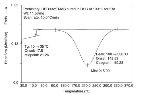
Figure 3. DSC at 10°C/min of epoxy-amine partially cured for 5 hours at 100°C. From [1].
Heat flow out of a material is exothermic; thermoset cure is an example of an exothermic process. Note that in a DSC plot the endothermic direction can be either up or down. A Perkin Elmer power-compensated DSC was used to obtain the data in Figure 2, where the exotherm in this case is downward. Note in Figure 3, the Tg is measured to be 21°C (using DSC midpoint) and the residual exotherm is measured at -59.3 cal/gram.
For each curing temperature and specified time, a DSC trace like that shown in Figure 3 is obtained. Once all the isothermal curing experiments are completed, the DSC traces are analyzed to determine Tg and ΔHres. The DSC fractional conversion is calculated using the equation above. Subsequently, the Tg and fractional conversion is plotted for each curing time and temperature to build the Tg-conversion plot over the entire Tg range.
Another method to cure the samples is to make the required number of DSC pans depending on how many isothermal cure times at each temperature and place them in an large aluminum weighing pan or a ceramic “dimple dish.” The image below shows an example of a porcelain plate with 12 depressions (“dimples”) that nicely hold the DSC pans in the oven during isothermal curing. A Sharpie pen can be used to note the curing times next to each depression.

[source: PZRT 12 depressions porcelain spot plate at Amazon.com].
Use one porcelain plate for each curing temperature. The curing may be done at various isothermal temperatures using a well-controlled oven (optimally using an oven with a nitrogen purge). At various time intervals, quickly open the oven and carefully remove a DCS pan. I like to place the DSC pan on the lab bench to quickly cool the DSC pan and then insert each DSC pan into a small plastic sample bag or envelope and note the curing temperature and time. Once the samples have been collected at each isothermal temperature, the DSC is used to measure the Tg and the ΔHres. After all the curing times and temperatures have been analyzed, then the Tg versus fractional conversion plot may be constructed.
Leave a Reply