Guest Post by Dr. R. Bruce Prime and Dr. John Avila
In this post we illustrate the p1 form described in Part 11 of this series by fitting conversion – rate of conversion data to a phenomenological equation based in chemical kinetics that is commonly used to describe autocatalytic cure kinetics. Such data can be measured by DSC although in these examples we generate the data mathematically as outlined previously.
Analyses utilizing this equation, discussed in detail in Part 10 of this series, will primarily benefit users who purchase thermosetting materials but do not have access to their chemical makeup.
The purpose here is to validate our computational schemes and to illustrate the utility of mathematically analyzing thermoset cure data. Our approach is to generate perfect data from Eq. 1 with a selected set of experimental parameters, add noise to simulate actual laboratory data, fit these noisy data to Eq. 1 and compare the computed results with the selected input parameters. A detailed description of the computational process is given in the Appendix. Three types of input data are examined: one with perfect data (ie no noise added), one set of data with a moderate level of noise, and one very noisy data set. Noise is added as described in Part 11 of this series.
The selected parameters are shown in the second column of Table 1. This is a simple system where m and n values are those expected from epoxy – amine chemistry and k2 is 100 times larger than k1. This is identical to the Small catalyst level example in Part 12 of this series and describes a system that is mostly autocatalytic in nature with about a 1% influence of external catalysis.
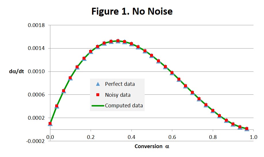
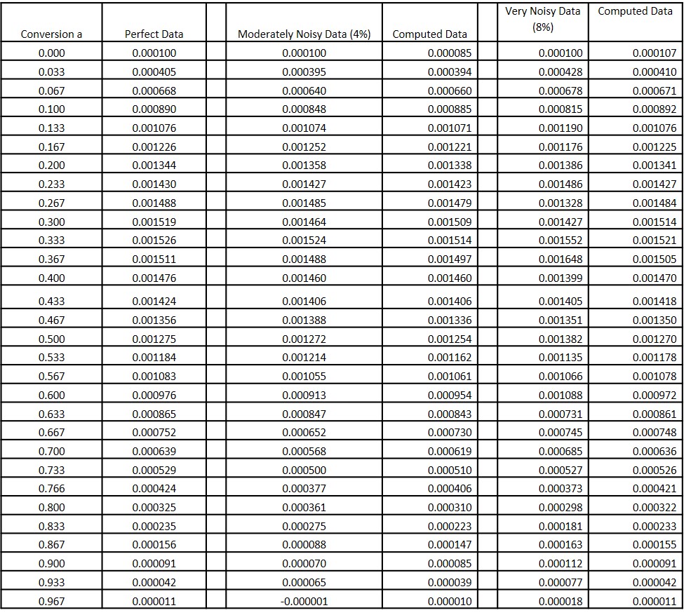
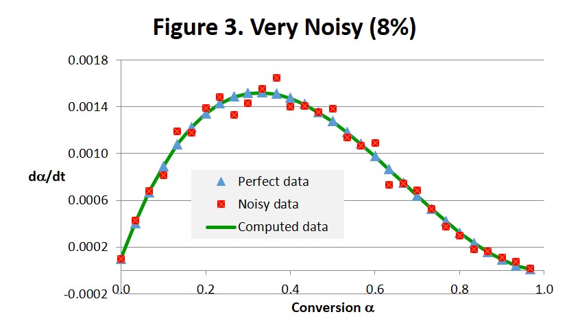
Rate of conversion (dα/dt) data is tabulated in Table 2 and plotted as Perfect data, Noisy data and Computed data. While we do not show units for rate of conversion note that they will be the same as the rate constants. For example, if k1 and k2 have units of sec-1 then these dα/dt values will be in sec-1. Perfect data is dα/dt computed from Eq. 1 with the selected parameters, Noisy data is Perfect data + Noise, and Computed data is generated by fitting the Noisy data to Eq. 1 and plugging those parameters back into Eq. 1. Table 1 contains the kinetic parameters affiliated with various stages of computation. The last three columns are discussed below. The sum of the squares, described in the Appendix, is a measure of the goodness of the fit to the simulated cure data, ie the noisy data.
Case 1, No Noise
The first column of Table 2 contains conversion values between 0 and 1 in equal increments determined by the number of data points, 30 in these examples. In the second column are Perfect Data computed from Eq. 1 without any added noise. In this case the Noisy data are identical to the Perfect data as expected, since no noise was added. The Computed results were also found to be identical to the Perfect data, and the computed parameters in the No Noise column of Table 1 were identical to the actual or input values even though the starting point values for k1 and k2 were each set to zero. These results combined with the perfect overlap seen in Fig. 1 and the exceptionally low value for the sum of the squares (essentially zero) all lend confidence to our computational schemes.
Table 1. Kinetic Parameters
Table 2. Conversion and Rate of Conversion Data for Three Noise Levels. Data in the Rightmost Five Columns are Rate of Conversion dα/dt
Case 2, Moderate Noise
The third column of Table 2 contains the moderately noisy data for the rate of conversion. Data such as these might be expected from careful experimentation with a well-maintained modern DSC. These data were fit to Eq. 1 as described earlier, giving the Moderate Noise results shown in Tables 1 and 2. Values for m, n and k2 are within a few percent of the input values. While k1 shows the most variation it has only a minor effect on the overall results due to its small value vis-à-vis k2.The 4th column of Table 2 contains rate data computed from Eq. 1 with the Moderate Noise parameters. While the data in Fig. 2 are not superimposed right on top of each other as in Fig. 1, the three sets of data can be seen to correspond remarkably well, especially the Computed data with the Perfect data. The sum of squares value of 3.8 x 10⁻⁸ compares favorably with the 1-sigma estimate of 3.9 x 10⁻⁸ in the Appendix, confirming a good fit of the computed data to the noisy simulated cure data.
Case 3, Very Noisy
The fifth column of Table 2 contains the Very Noisy data for the rate of conversion. Data such as these might be expected from less careful experimentation or with a not well-maintained or older and less sensitive DSC. These data were fit to Eq. 1 giving the Very Noisy results shown in Tables 1 and 2. The sixth column contains rate data computed from Eq. 1 with these Very Noisy parameters. From Table 2 and Fig. 3 these results can be seen to be much closer to the Perfect Data than to the Very Noisy data. Thus even though the simulated data are quite noisy the fit to Eq. 1 is nonetheless quite good as can be seen by the virtual overlap of the Computed data with the Perfect data in Fig. 3. The sum of squares value of 1.4 x 10⁻⁷ vis-a-vis the 1-sigma estimate of 1.55 x 10⁻⁷ in the Appendix supports this conclusion.
To summarize, even with noisy cure data we can expect a good fit to the underlying relationships governing the cure reaction. With its unique ability to independently measure both conversion and rate of conversion DSC is ideally suited to characterize cure processes. In the real world of actual cure data we can anticipate the ability to model cure reactions with good predictability. The k2 values for both the Moderate and Very Noisy cases are sufficiently reproducible to be used in an Arrhenius plot of ln k2 vs. T-1 to estimate the activation energy from data taken at multiple temperatures.
This concludes our current series on Thermoset Cure Kinetics. Future posts will focus on the kinetic analysis of conversion – time data, which can be generated by a number of techniques including DSC and FTIR and Raman spectroscopies, and the incorporation of temperature as a variable.
Appendix: Fitting data.
In Equation 1 we start with a set of α values. In our experiments, we picked a uniformly spaced sample of conversions between 0 and 1. In addition we chose values for the 4 parameters: , , m and n that are used to generate the “perfect” dα/dt and the noisy dα/dt as described above. We then let the 4 parameters be unknowns and try to recover those values using a numerical least squares process. This process consists of starting with an approximation to the “unknown” parameters and iteratively modifying them to minimize the sum of the squares of the differences between the noisy dα/dt values and the “perfect” dα/dt values obtained from Eq. 1 with the estimated parameters. There are libraries of excellent software routines for such problems and we used the method in reference [1].
As part of the computation we display the sum of the squares of the differences between the noisy dα/dt and the computed dα/dt in Table 1. The noise values that are used for each data point are of the form:
where r is a random variable with standard deviation σ representing the noise level (e.g. 4% or 8%) and (dα/dt)mean is the average value of dα/dt. We would expect the sum of squares to be approximately n times the noise level squared where n is the number of data points. If we replace r by in the equation, we obtain a 1-sigma estimate for the sum of squares. If we have minimized the sum of squares, we would expect its value to be no larger than this 1-sigma estimate. On the other hand, if the sum of squares exceeds the 1-sigma estimate by a significant amount, then we probably have not minimized the sum of squares. In the cases shown in Table 2, the mean value for dα/dt is approximately 9 x 10⁻⁴ and there are 30 data points. This yields a 1-sigma estimate for the sum of squares of 30(σ x 9 x 10⁻⁴)2 which is 3.9 x 10⁻⁸ for σ = .04 and 1.55 x 10⁻⁷ for σ = .08. Such values would indicate a high degree of confidence for the computed parameters.
References
[1] Commons Math: The Apache Commons Mathematics Library, https://commons.apache.org/proper/commons-math/


Leave a Reply