Guest Post by Dr. R. Bruce Prime and Dr. John Avila
This post outlines the mathematical approaches to model the cure behavior and then analyze the cure data to extract kinetic parameters. We do this by utilizing equations developed in the previous post that model the cure path of autocatalytic systems like epoxy-amine.
- Modeling Cure Behavior
For this case we developed relatively simple software routines for generating and plotting conversion – time and rate of conversion – time data from chemically based equations. The objective is to explore thermoset cure behavior such as the effects of stoichiometry and added catalyst. We generate the data as follows. We start with an equation that models the behavior of interest. We then choose appropriate parameter values and numerically compute conversion and rate of conversion at a selected number of points or times. We make use of Eq. 2 in the previous post (Eq. 1 in this post), a detailed equation based on the chemistry of the cure reaction that is able to explore how stoichiometry may affect the cure path.
dαEp/dt = (k1 + k2 αEp )(1-αEp)(B-αEp) (1)
where dαEp/dt is the rate of conversion of epoxide, αEp the fractional conversion of epoxide and B the ratio of amine hydrogen equivalents to epoxide equivalents. Remember that the amine concentration αAm is represented by the term (B-αEp), k1 is the rate constant for the externally catalyzed reaction and k2 is the rate constant for the autocatalyzed reaction. Equation 1 will be used to model the effects of stoichiometry in Part 13.
For applications where the stoichiometry is balanced, B = 1 and αEp = αAm = α, where α is the overall conversion in an amine-epoxide system and equation 1 simplifies to:
dα/dt = (k1 + k2 α)(1-α)2 (2)
In the case of epoxide reacting with amine recall that the term (1-α) represents the concentration of reactants, for example, the epoxide and the amine and that α represents the concentration of catalyst generated in the reaction, for example, hydroxyl functionality. Addition of external catalyst can be modeled by increasing k1 and is the subject of the next post.
- Analysis of Cure Data
This case is more complex where our ultimate intention is to analyze actual cure data. In the absence of such data we generate “typical” cure data and then fit them to Eq. 3 below. Here we address the generation of data for ‘model’ autocatalytic systems in one of two forms:
- (p1) conversion vs rate of conversion data, typically generated by isothermal DSC which is uniquely capable of simultaneously measuring both of these parameters.
- (p2) conversion vs time data, which may be generated by a variety of techniques including DSC, FTIR and Raman spectroscopies.
In particular we examine the analytical approach by generating data in one of these two forms with appropriate noise values such as one might observe in laboratory conditions. In each of these two forms, the assumption is that there is an underlying equation that models the data. Equation 3 is such an equation (from (2), where reaction orders m and n are treated as variables [1,2]. It has four parameters (k1, k2, m and n) that can be adjusted to best fit the given data. Generally, these parameters enter into the equations in a nonlinear manner which makes an analytical approach to their estimation usually impossible. Fortunately there are good numerical methods for these problems [3].
dα/dt = (k1 + k2 αm) (1-α)n (3)
A common approach is to estimate the cure parameters (rate constants and reaction orders), measure the discrepancy between the data and the values predicted by the model equation, make appropriate changes to the estimated parameters, and repeat. In the least squares formulation, we attempt to minimize the sum of the squares of the discrepancies over all the data points.
Generation of simulated cure data
For the demonstration examples in this blog series we have generated data as follows. We first start with Eq. 3. We then choose parameter values and numerically compute the conversion and conversion rates for the given model at a number of points. To these values we then add “noise” represented by a normally-distributed random number with zero mean and a variance which we can specify. The resulting data are then treated as the input to the least squares algorithm and the goal is to see how well we can recover the parameters used to produce the pre-noisy data. In the course of exercising these algorithms we have observed that the preferred settings for the estimated starting values are k1 = k2 = 0, m =1, and n = 2.
The p1 form
First we consider the p1 form. The data consists of pairs ( α and dα/dt) at specific (but unspecified) values of time, where α is the conversion and time is given by t.
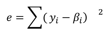
For the model, we use Eq. 3, a phenomenological equation based on epoxy-amine chemistry [1,2]. If we let yi denote the “measured” rate of conversion corresponding to αi, ie the data with noise, and we let βi be the value of the rate of conversion obtained for αi and a particular set of approximate parameter values, then we wish to minimize the value of e as given by:
(4)
This is the so-called least squares problem. The goal is to recover the parameter values used to generate the model data. This subject is addressed in Part 14 of this series.
The p2 form
In the p2 form, the subject of Part 15 in this series, we are given data pairs of the form (ti, αi). Assuming the same model as given above, the least squares problem is the same except that there is a wrinkle: βi is not computable directly as in p1. Instead, each time the value of any of the parameters is modified, one must solve the differential equation that models the data. There is a numerical software library [3] that we have used effectively to solve both forms. In general, the solution in the p2 form is substantially more computationally intensive.
Rationale
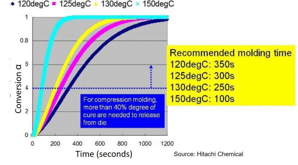
Let’s look at a practical example of the type of thermoset curing where modeling would be very important. In this case, an epoxy mold compound (EMC) used in a new type of electronic package (called fan out wafer level package) is compression molded. The gel point (αgel) occurs at a conversion of approximately 40%. During the compression molding process, the EMC must be cured to at least the gel point so the part will have dimensional stability after the molding process. In Figure 1, the Hitachi recommendation is that the degree of cure be at least 40% prior to releasing from the mold. Figure 1 shows that with increasing mold temperature, the time to reach 40% conversion decreases. At a mold temperature of 150°C the molding time is 100 seconds versus 350 seconds for a mold temperature of 120°C. After mold release, the EMC is gelled but not fully cured, requiring a second post mold bake step. From a manufacturing throughput perspective, the time in the mold is optimized to achieve the required 40% conversion and minimize warpage on cooling.
Figure 1. Degree of cure (conversion) as a function of time for various mold temperatures for an epoxy mold compound (source: Hitachi Chemical)
Numerical results
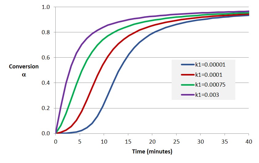
The example shows the importance of modeling the conversion versus time relationship for thermoset curing. In subsequent posts examples will be presented showing how the approaches discussed here are used to generate conversion-time plots as shown in Figure 2. Note the similar shape of the modeling results with the data in Figure 1.
Figure 2. Degree of cure (conversion) as a function of time for various model parameters
References
- K. Horie et al., J. Polym. Sci., Polym. Chem. Ed. 8, 1357 (1970).
- S. Sourour and M. R. Kamal, Thermochim. Acta 14, 41 (1976).
- https://commons.apache.org/.


Leave a Reply